The Richtmyer–Meshkov instability is a fluid instability that develops when a shock wave passes through a perturbed interface separating fluids of different densities. The initial disturbance grows into rising bubbles and narrow spikes, and eventually develops into a turbulent mixing layer filled with structures across many different spatial scales.

For our final project in CS 6635: Visualization for Scientific Data at the University of Utah, Dhruv Ram and I explored how different scientific visualization techniques could reveal these structures inside a high-resolution Richtmyer–Meshkov simulation snapshot. The project was also featured in the University of Utah Center for High Performance Computing (CHPC) Research Highlights.

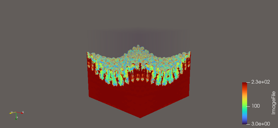
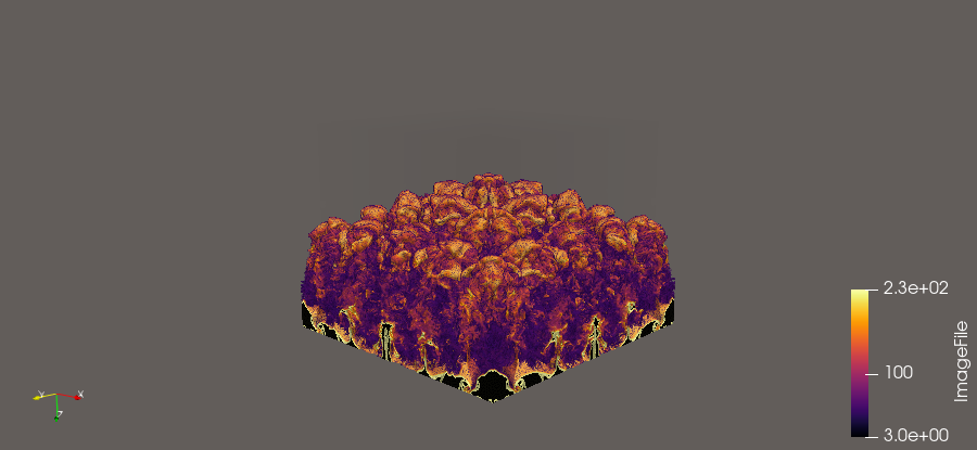
Direct volume rendering (L) and Volume Rendering subset (R) of the turbulent mixing layer

The Dataset

The dataset is an entropy field from a Richtmyer–Meshkov instability simulation, obtained from the Open SciVis Datasets collection. It contains a single three-dimensional snapshot at simulation timestep 160, when the instability has already developed into a complex turbulent mixing region.

The raw volume has a resolution of 2048 × 2048 × 1920 with one unsigned 8-bit entropy value per voxel. This corresponds to more than 8.05 billion voxels and approximately 7.5 GiB of uncompressed scalar data. Once loaded into a visualization application, additional memory is also required for derived fields, transfer functions, geometry, and rendering buffers.

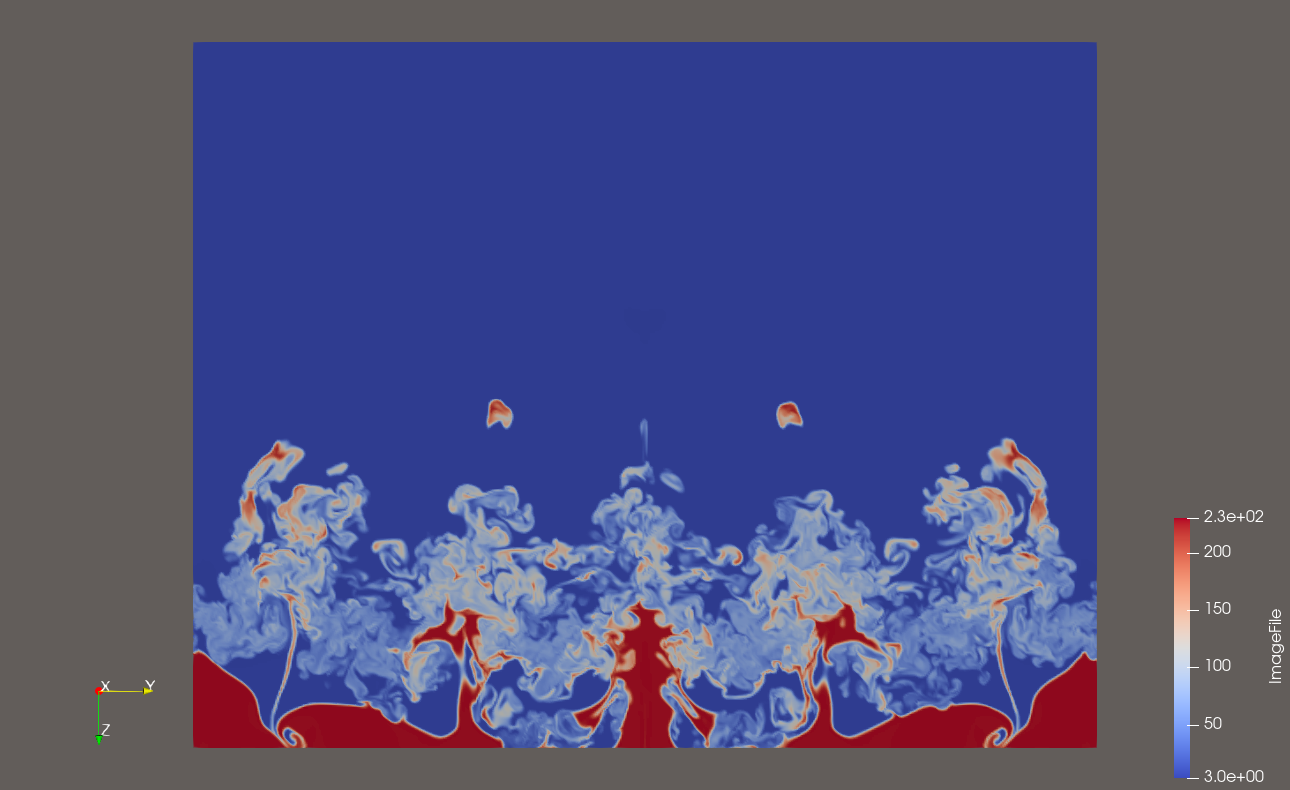
A planar slice through the entropy field reveals the dense, irregular structure of the mixing layer

The input was distributed as a headerless RAW file, so its dimensions, scalar type, and byte ordering had to be specified explicitly when importing it. I converted the volume into VTI format to preserve this metadata and make it easier to reopen the dataset and build repeatable ParaView pipelines.

What Makes the Instability Interesting?

When the shock crosses the perturbed density interface, the pressure gradient and density gradient are not perfectly aligned. This deposits baroclinic vorticity at the interface and amplifies the original perturbations. Heavy fluid penetrates the lighter fluid as spikes, while the light fluid rises into the heavier fluid as bubbles.

At later stages, these structures stretch, roll up, interact, and break into progressively smaller features. This makes the dataset a useful visualization challenge: a single image must communicate both the overall shape of the mixing layer and the fine turbulent structures inside it.

No single technique showed every part of the data equally well, so I built several complementary ParaView pipelines:

• GPU-accelerated direct volume rendering
• Isosurface extraction using the Contour filter
• Orthogonal slices and animated slice sweeps
• Scalar-gradient computation and glyph visualization
• Global illumination and volumetric scattering experiments

GPU Volume Rendering

Direct volume rendering was the most complete view of the dataset because it preserves the full three-dimensional scalar field instead of reducing it to a surface. I used ParaView's GPU ray-casting volume mapper with composite blending and designed a transfer function that mapped lower and higher entropy values to distinct colors and opacities.

The opacity transfer function was especially important. Assigning too much opacity to the full range quickly hid the interior, while a very sparse transfer function removed the context needed to understand the overall mixing region. The final mapping kept low-opacity material around the volume while emphasizing the entropy ranges containing the most visible turbulent structure.

GPU ray-cast volume rendering using a custom color and opacity transfer function

To focus the view, I isolated approximately the middle 60% of the dataset containing the turbulent mixing layer. Removing relatively empty regions reduced visual clutter and allowed the available screen space and GPU memory to be concentrated on the most important structures.

Global Illumination and Volumetric Scattering

Standard volume rendering made the entropy distribution visible, but dense regions could still appear visually flat. I experimented with ParaView's global illumination reach and volumetric scattering controls to introduce stronger depth cues.

Global illumination improved the separation between overlapping structures by adding soft self-shadowing through the volume. Volumetric scattering created a more cinematic result in which light appeared to travel through and interact with the participating medium. These effects were useful for presentation, although they had to be balanced carefully: excessive scattering could obscure the scalar relationships encoded by the transfer function.

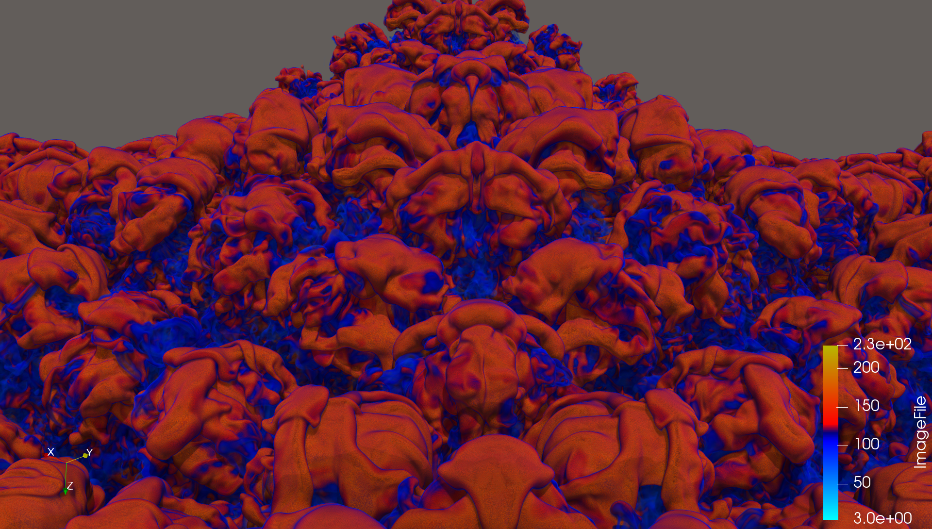
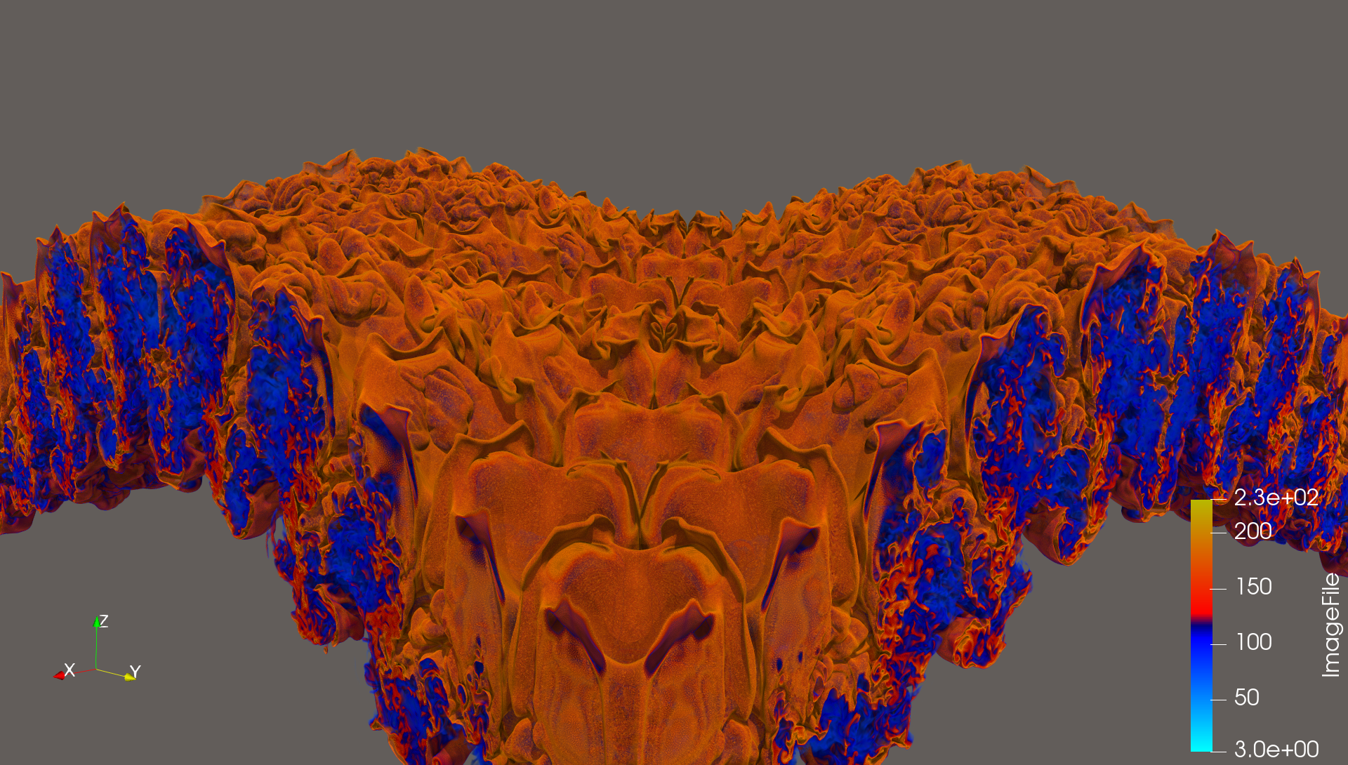
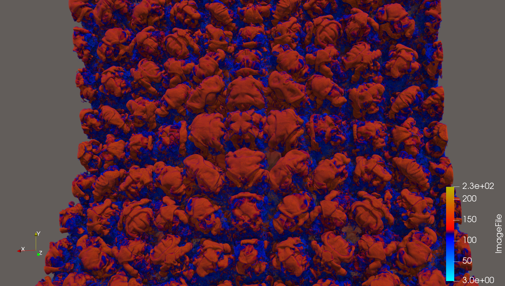
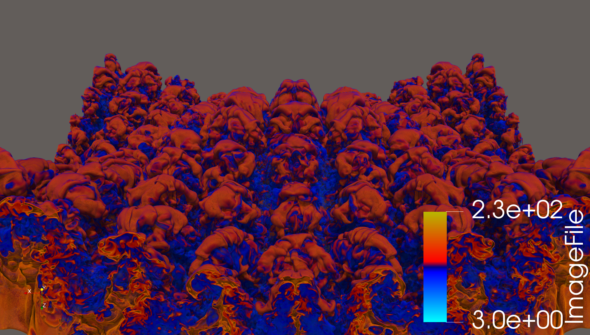
Global illumination (L) improves depth separation, while volumetric scattering (R) produces a softer participating-medium appearance

Extracting Isosurfaces

Volume rendering provides context, but it can be difficult to identify a precise scalar boundary inside a translucent volume. To obtain a clearer geometric representation, I used ParaView's Contour filter to extract a surface at an entropy value of 116.5.

The extracted isosurface turns a selected entropy level into explicit geometry. With computed normals, low opacity, and a separate color transfer function, it reveals folds, sheets, and connected turbulent structures that are harder to distinguish in the full volume rendering.

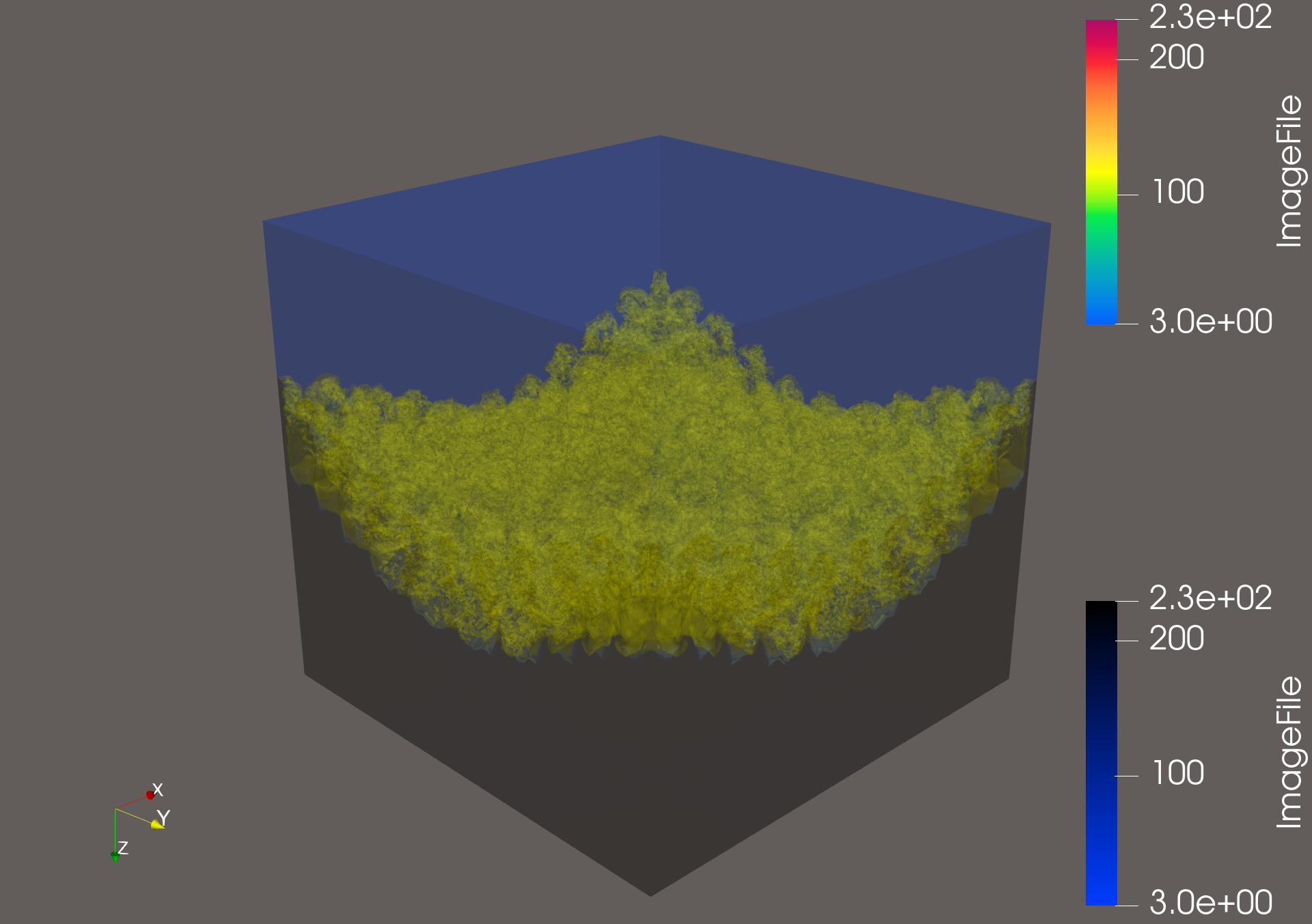
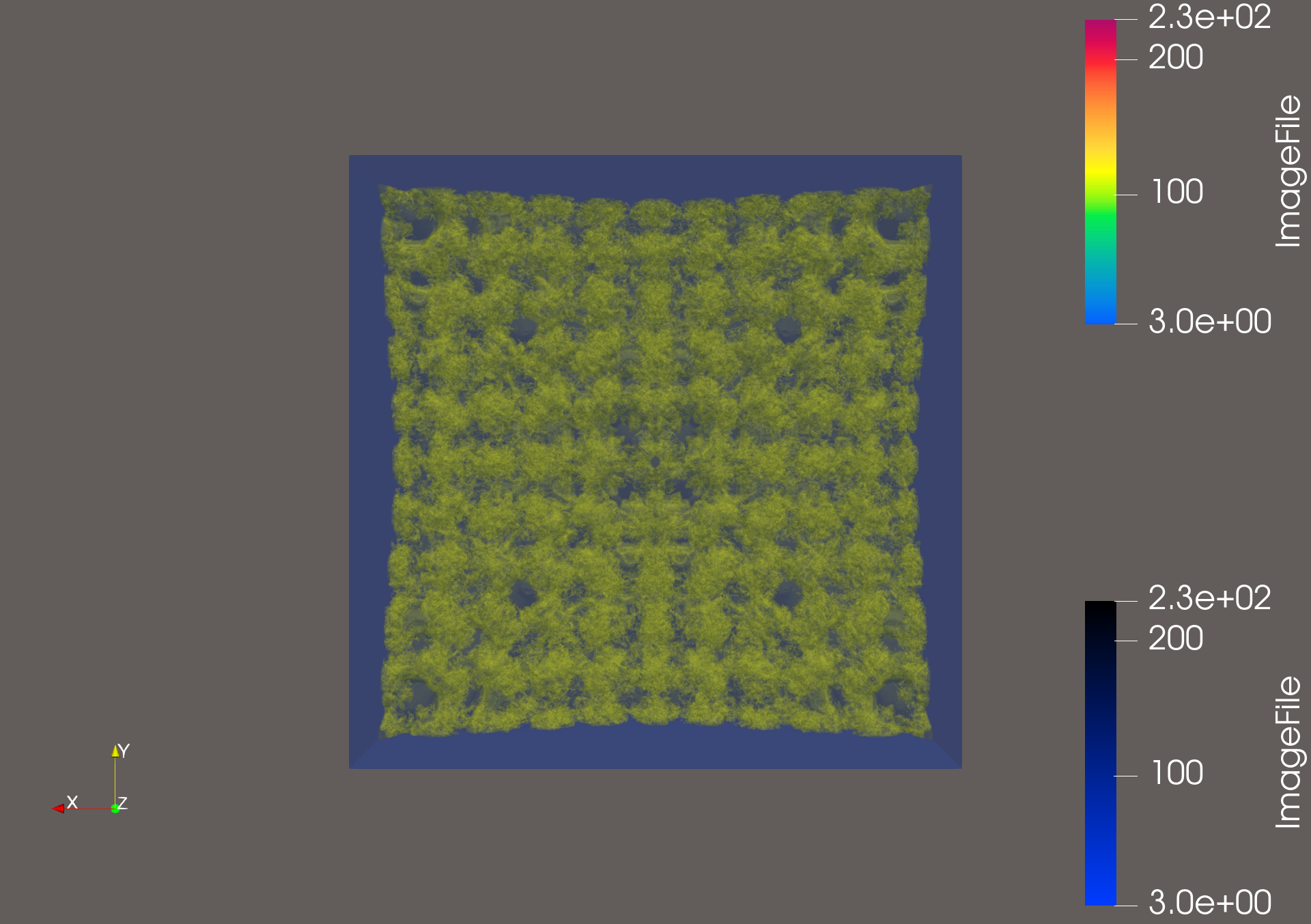
Entropy isosurface at 116.5 with the original volume retained as translucent context

I kept the original VTI volume visible behind the surface at low opacity. This combination worked better than either representation alone: the contour supplied a clear geometric boundary, while the volume preserved the spatial context around it.

Slices Through the Volume

Slices provide a direct view of the original scalar samples without the occlusion and opacity choices involved in volume rendering. I created slices along the X, Y, and Z axes to inspect how the instability changes across the domain.

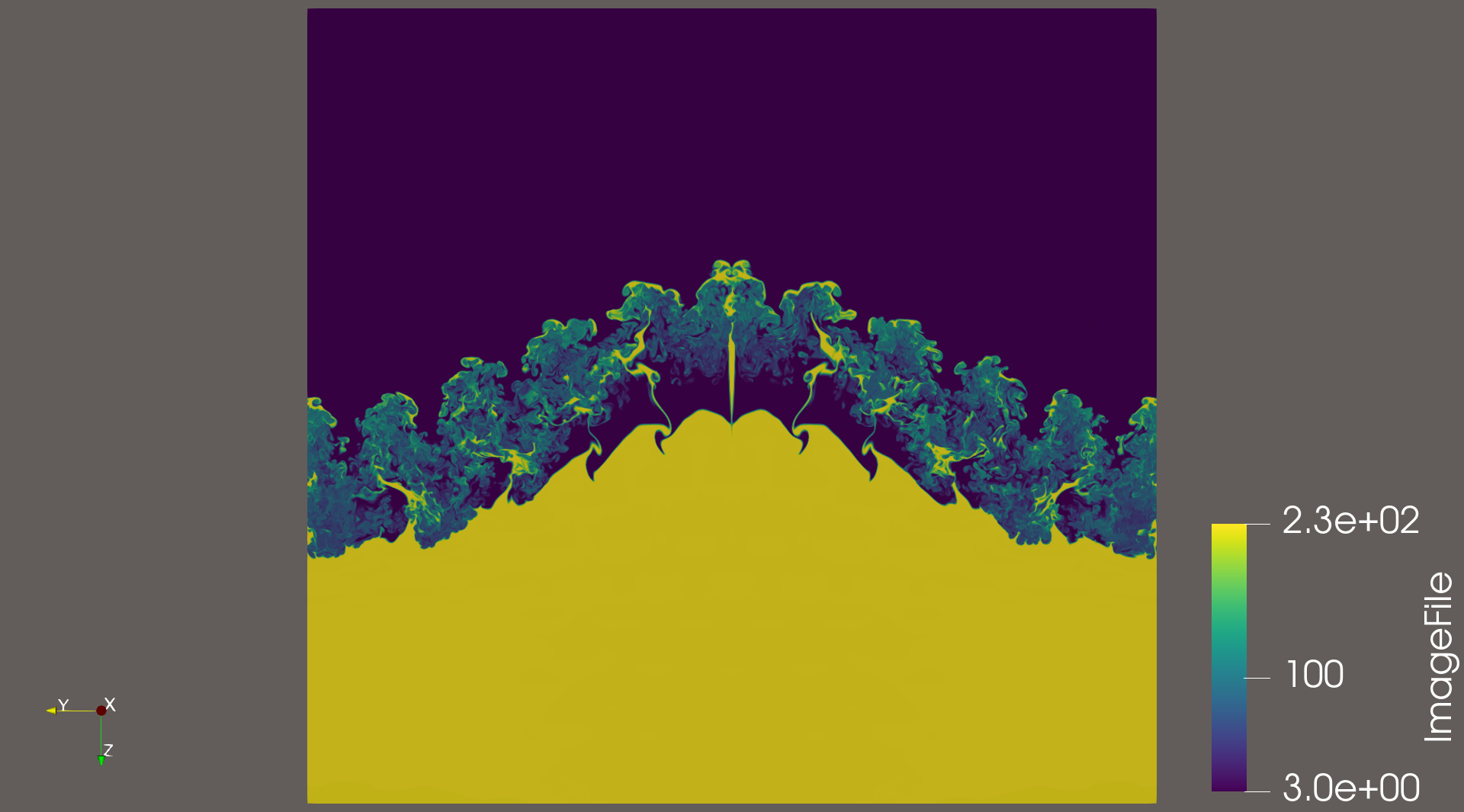
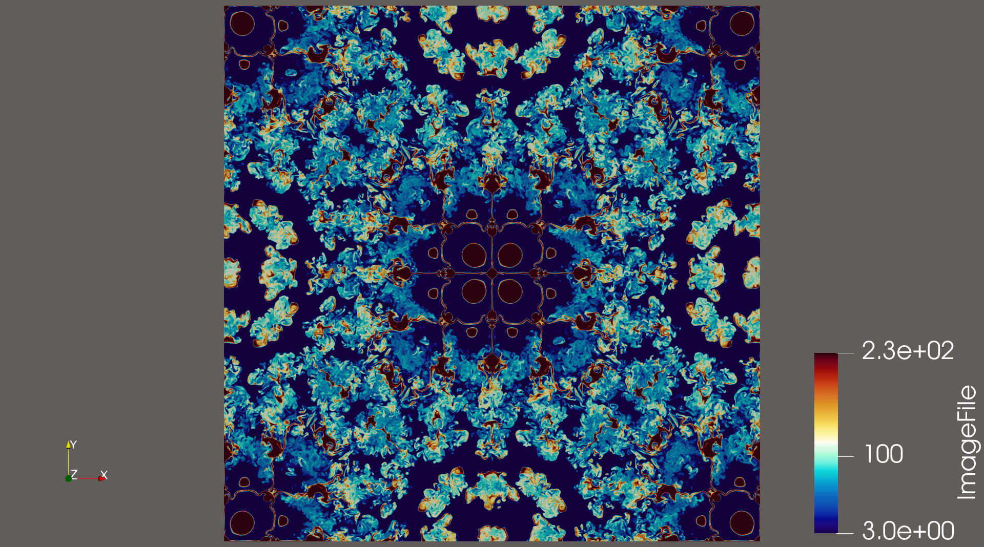
Orthogonal slices expose internal entropy variations that are hidden in an exterior view

Because the source contains one timestep rather than a temporal sequence, the animation does not show the simulation evolving over time. Instead, I animated the slice origin through the volume. This produces a spatial scan that makes it possible to follow structures through depth and observe where features merge, split, or disappear.

Animated slice sweep through the three-dimensional entropy field

Visualizing Scalar Gradients

I also computed the gradient of the entropy field and sampled it with glyphs. The gradient points in the direction of the strongest local increase in entropy, while its magnitude indicates how rapidly the scalar value changes.

This makes gradient glyphs useful for identifying sharp interfaces and regions of strong local variation. Since the source data contains entropy rather than velocity, these glyphs should not be interpreted as fluid trajectories or flow direction; they describe the structure of the scalar field itself.

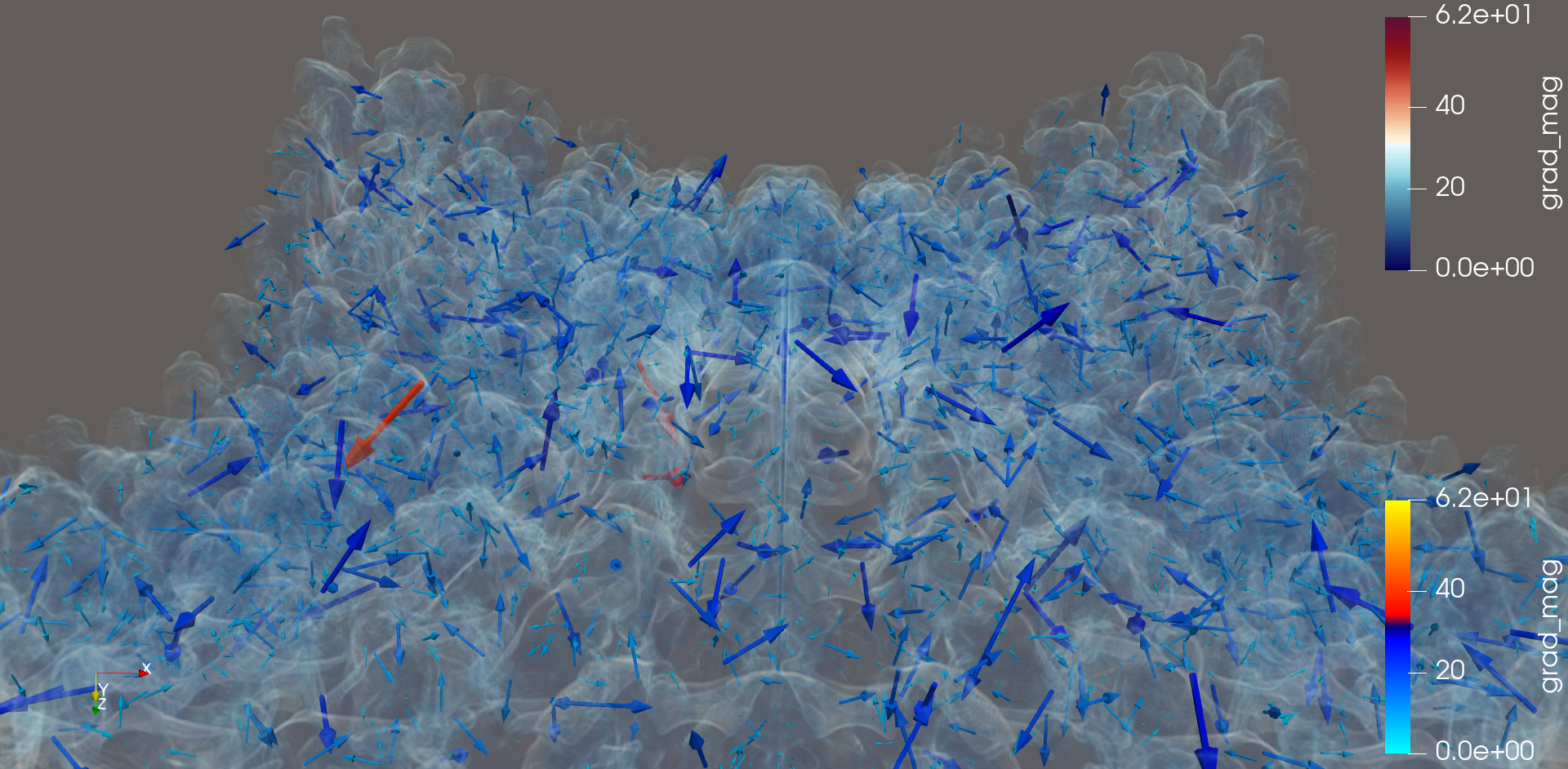
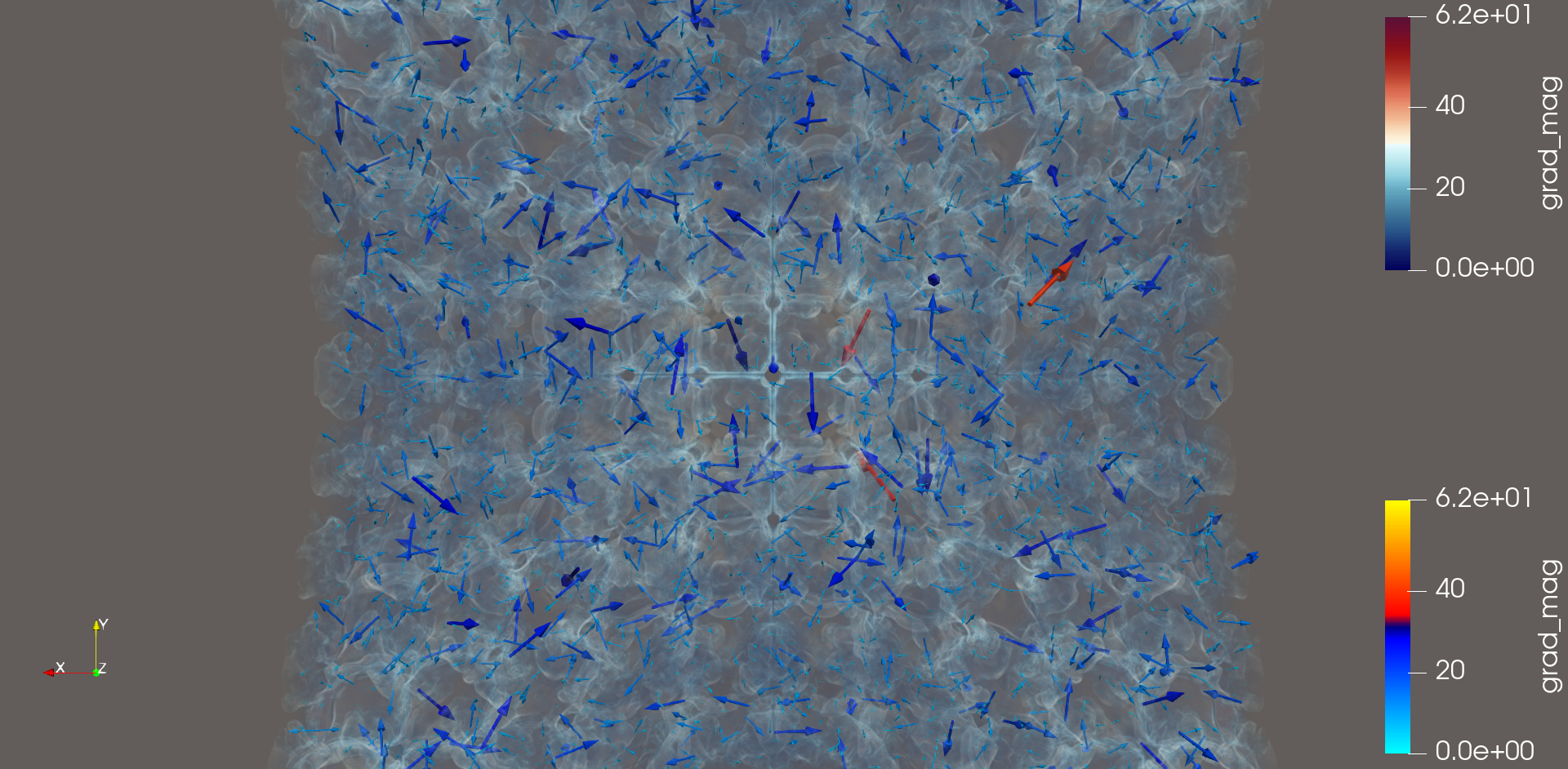
Sampled entropy-gradient glyphs highlight sharp transitions around the mixing interface

Glyph density had to be reduced substantially because placing an arrow at every voxel would be both computationally impractical and visually unreadable. Sampling the field created a much clearer view of the dominant directions of local entropy change.

Moving the Workflow to CHPC

The full-resolution dataset exceeded what was practical to explore on a typical local workstation. Even though the RAW file itself is about 8 GB, volume rendering requires additional GPU memory for textures and intermediate data. Early attempts encountered memory pressure and failures while allocating the complete volume texture.

I moved the workflow to the University of Utah's Center for High Performance Computing. ParaView ran inside a containerized environment with EGL for headless rendering, allowing the visualization to use NVIDIA A40 GPUs without depending on a physical display or a conventional X server.

The remote workflow combined:

• CHPC interactive desktop sessions for setup and inspection
• A containerized ParaView environment for reproducibility
• EGL-based offscreen rendering on NVIDIA A40 GPUs
• pvserver for remote computation and rendering
• SSH tunneling for interactive client-server access

This setup moved the expensive data processing and rendering close to the dataset while still allowing the scene to be explored interactively from a local machine. It also turned the infrastructure work into an important part of the project: at this scale, how the visualization is deployed matters almost as much as the filters used to create it.